
Content Management - First post with RMarkdown
This article is Part 8 in a 8-Part series called Content Strategy.
- Part 1 - Content Management - Introduction
- Part 2 - Content Management - Useful Tools 1 - Markdown
- Part 3 - Content Management - Useful Tools 2 - Basic Web
- Part 4 - Content Management - Useful Tools 3 - No Mr Hyde!
- Part 5 - Content Management - Syntax Highlighting
- Part 6 - Math Integration
- Part 7 - Content Management - knitr and RMarkdown integration
- Part 8 - This Article
Introduction
At the end of the previous post we went through a diverse range of some of the ways to incorporate the RMarkdown content into my website. The path that I settled on was knitr-jekyll, since it looked fairly simple to import into my workflow.
Result: Cooking with gas!
Now that we are pretty much setup, let’s see how it all works on some simple data. Below is the first chunk in our analysis, which sets things up for us. We will be looking at the pressure dataset, which is included in the datasets package that comes with the core distribution of R.
In this case, the setup is pretty simple and self explanatory.
# obtain the dataset
data(pressure)
# display the first couple of rows
head(pressure)
## temperature pressure
## 1 0 0.0002
## 2 20 0.0012
## 3 40 0.0060
## 4 60 0.0300
## 5 80 0.0900
## 6 100 0.2700Displaying tabular data
I have used the kable() function from knitr to good effect in the past to create some nice tables. Typically, I don’t bother specifying any other arguments besides the dataset, but today we will dabble a little ![]() .
.
# displaying the same dataset using knitr's kable() function to format it nicely.
# base caption with table description.
pressureDataCaption = "Brief Snapshot of the Pressure dataset"

# constructing table with modified caption
# optionally, we could specify a format such as pandoc. see ?knitr.kable
knitr::kable(head(pressure), format = "html", caption = paste(pressureDataCaption, "with kable() from the knitr package."))| temperature | pressure |
|---|---|
| 0 | 0.0002 |
| 20 | 0.0012 |
| 40 | 0.0060 |
| 60 | 0.0300 |
| 80 | 0.0900 |
| 100 | 0.2700 |
Alternatively, one could use the pander package. I found an example of this while looking at the SciViews website, which interestinly uses Jekyll and servr ![]() .
.
# alternatively, one could use the pander() function from pander.
require(pander)
## Loading required package: panderpander::pander(head(pressure), caption = paste(pressureDataCaption, "with pander() from the pander package."), style = "rmarkdown")| temperature | pressure |
|---|---|
| 0 | 2e-04 |
| 20 | 0.0012 |
| 40 | 0.006 |
| 60 | 0.03 |
| 80 | 0.09 |
| 100 | 0.27 |
Table: Brief Snapshot of the Pressure dataset with pander() from the pander package.
RStudio formats the table content a little better, but this will do nicely… need to work on that a bit later on though.
Displaying plots
Now for the really interesting part… plotting graphics ![]() . This section contains a simple comparison of the base plotting system with that of ggplot2. This is probably the most challenging thing about knitting documents in R, because:
. This section contains a simple comparison of the base plotting system with that of ggplot2. This is probably the most challenging thing about knitting documents in R, because:
- the figures need to be generated and stored in the correct location
- the figures need to be referred to properly within the created document
Needless to say, this was an exciting development when this worked ![]()
Note: I randomly found this stackoverflow question on embedding existing graphics in knitr chunks. I don’t need this now but it might come in handy. Remember…
“It is better to have it and not need it… than to need it and not have it”
Base ploting system
An example of a pretty basic but informative plot produced using the base plotting system (R’s simple default).
# a simple plot of the data
plotTitle = "Pressure Dataset: Plot of Pressure and temperature"
plotAxes = c(x = "Temperature", y = "Pressure")
plot(pressure$temperature, pressure$pressure, main = plotTitle,
    xlab = plotAxes[['x']], ylab = plotAxes[['y']])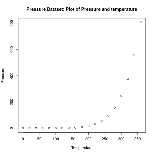
ggplot2 ploting system
The same information displayed using the ever popular and highly potent ggplot2.
library(ggplot2)
pressureFig = ggplot(data=pressure) + aes(x=temperature, y=pressure) + geom_point(color = "blue") + theme_minimal() + labs(title = plotTitle, x = plotAxes[['x']], y = plotAxes[['y']])
pressureFig
Setup
That was a nice and simple walkthrough to show how RMarkdown data can be processed and incorporated neatly into a Jekyll-based web authoring framework. More importantly, this is essentially a first test of getting knitr-jekyll integrated into my system.
The obvious question is: “how did you do this?”. I deliberatly left this to last because I wanted to demonstrate the results of the process as a justification (of sorts) for the effort invested before describing how this was achieved.
I basically followed the strategy that I discussed previously, making modifications as I went. The steps to create the current setup were:
- Install the servr R package
- Create the
_source/subdirectory for RMarkdown version of posts to process- included a
_source/helper_scripts/subdirectory to house the helper scripts that I need - the first helper file
process_posts.Rcontains theprocess_rmd_posts()function, which is basically a wrapper ofservr::jekyll()with a custom jekyll command (I prefix with “bundle exec” due to my present config and I sometimes work with drafts or future posts). The most important change is that I set theserveparameter to false (i.e.serve=F). This was because RStudio crashes everytime I try to build using the default option of true . However, this isn’t a problem for me as I don’t want to serve the website in RStudio anyway and use a web browser instance instead
  .
.
- included a
- Imported the original build.R code and made modifications (compare with my current version here) during setup.
- images saved to the
images/fig/posts/subdirectory because I didn’t want to have another “top level” subdirectory devoted to images (originally calledfigure/), when theimages/folder housed all of my site graphics. Took a litle mucking around but it was worth it. This is setup so that any Rmd content with the pages layout can later be stored inimages/fig/pages/(still to work on that further). - Fixed an issue with figure image links where images were stored in the expected location but not properly linked in the document. I can only presume that this was due to how the
baseurlYAML variable was setup in the Jekyll Now_config.yamlfile.
- images saved to the
Conclusion
This is a really good start and I will work on dealing with processing drafts and pages later ![]() .
.
This article is Part 8 in a 8-Part series called Content Strategy.
- Part 1 - Content Management - Introduction
- Part 2 - Content Management - Useful Tools 1 - Markdown
- Part 3 - Content Management - Useful Tools 2 - Basic Web
- Part 4 - Content Management - Useful Tools 3 - No Mr Hyde!
- Part 5 - Content Management - Syntax Highlighting
- Part 6 - Math Integration
- Part 7 - Content Management - knitr and RMarkdown integration
- Part 8 - This Article